
In the first session of our Deep Learning series, we described the basis of our approach to Deep Learning: the classical theory of neural networks. In this second we will try to focus on more practical aspects, such as the use of hyperparameters.
One of the most fascinating ideas about Deep Learning is that each layer gets a data representation focused on the objective of the problem to be solved. So, the network as a whole generates an idea of each concept, derived from data. Some questions arise: “how are networks different from each other?” and “how can we build one that represents exactly what we want?” The answer to these questions resides in the hyperparameters used to construct the network.

Before we start, please allow me to remark the difference between parameters and hyperparameters: while hyperparameters represent the configurable values used when building the Net, parameters constitute the learnt values (weights) obtained while optimizing the loss function.
The very first doubt that comes to mind when building a neural net is the number of layers or units per layer that we will use. Unfortunately, here there are no magic numbers, but as a general advice, the complexity of the problem to be solved should give us an intuition to define the network architecture. For instance, when you have to distinguish among cat breeds you will probably have to configure a much more complex net than when distinguishing cats and pirates. So, in order to achieve that, complexity grows as the net grows.

If we think about images and we build an image recognition network, the very first layers will probably detect simple features like borders or straight lines. The next layers will be able to detect combinations of the previous features (e.g: picture frames). If we go even deeper into the network, it would even become possible to detect something as complex as a tiny brown muzzle with whiskers. So, the complexity of the problem is related to the size of the network (and please note, a large-sized net can only be trained with a large-sized amount of data).
Building a Deep Learning Network: understanding its hyperparameters
Besides units and layers, there are a few other important components. We will give an overview of the most important ones, but for a more detailed view, please allow me to redirect you to the video for this session.
Let’s start with the activation functions. In the last session, we studied the sigmoid function, which takes values in [0,1], as one of the most common activation units, but it is not the only one. Among the most popular ones stands the hyperbolic tangent, which ensures a smooth symmetric transition between positive and negative and has fair properties for intermediate layers, as its expected output has zero mean.
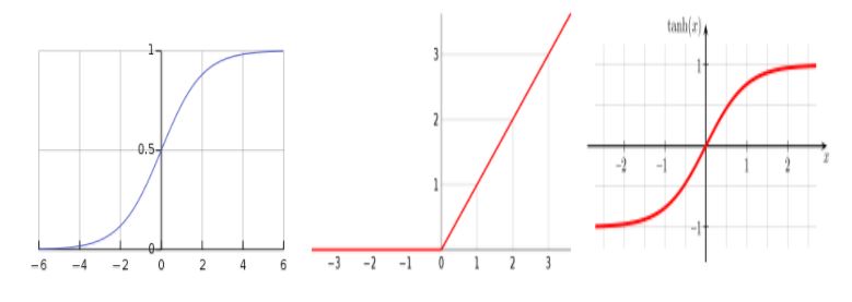
One of the requirements for this kind of functions is an easy differentiation, as the whole backprop process needs to compute and carry derivatives. Thus, it will help us avoid a lot of calculus (don’t worry, we can “trick” the relu function to act as differentiable).
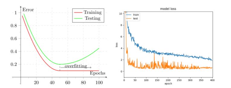
Another hyperparameter to be considered is, once the algorithm is chosen, the way in which it will be trained. Usually the training takes several data passes (epochs) and the number of epochs has to be adjusted: too few can lead to underfit, and too many to overfit. Of course, this is complexity-dependant, but once we have our network configured, we can keep track on both training and testing datasets of the loss along the epochs in order to get an idea of when to stop training.
In addition to the epoch number, it must be decided whether the weight update is done after each epoch, sample or fraction of samples (batch). In most cases, the data is divided in batches, and the batch size becomes another feature of the network, introducing the concepts of mini-batch and stochastic gradient descent.
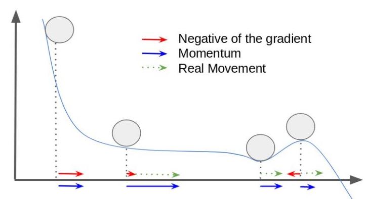
Another key hyperparameter is the optimization algorithm. As we have already seen, initialization is important, but some algorithms can help us, in certain cases, to recover from a previous wrong choice, modifying the way the parameters are updated, like for example, using momentum or not in order to skip local minima.
Besides the classic Mini-batch Gradient Descent, some of the most popular optimization methods are, for example, the RMSProp, which was originally proposed by Hinton, and the Adaptive Moment Estimation (Adam). Both can also take advantage of the aforementioned mini-batch partition.
When digging into the world of Deep Learning, one of the a priori weak points of the nets is their tendency to overfit. The representations built are data-based and the data on which they are based is the training set. Nevertheless, there are ways to reduce it, for instance, using regularization.
Some of the most classic regularization techniques within the machine learning field are the regularizations L1 and L2 and combinations between them. Both are also used in neural nets, in order to keep the parameter values under control. The use of mini-batches on the optimization algorithm is also another kind of regularization itself, but one of the most widely used reg techniques is the so-called Dropout. Essentially, it consists of randomly dropping some of the neurons on each pass. This idea makes the network more adaptable, eliminating some variance and getting a more adaptable, less overfitted model. The concept is similar to when, for example, a basketball player trains hopping on a single leg. He probably will not face this situation during a match, but he will gain balance and stability.
TensorFlow and Keras: easing the construction
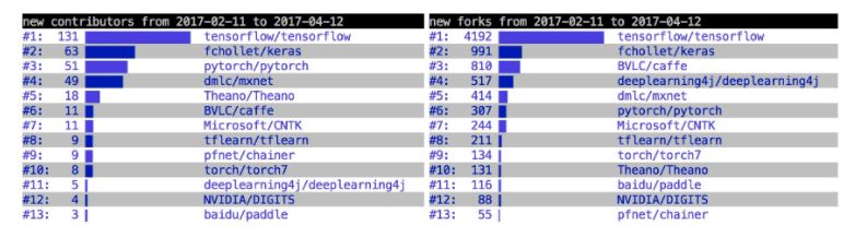
TensorFlow is one of the most widely used frameworks for Deep Learning. The whole Machine Learning community is aware and a large majority is trying it. It was developed by Google and technically is one of the most powerful frameworks in terms of performance. But it is also a little unfriendly, and when trying to initiate on Deep Learning, you may get stuck on the framework before understanding what you are doing. This is why there are some other “metaframeworks” like Keras. Using Keras makes life easier when building Deep Learning models.
Keras isolates users from the backend and allows the models to be constructed in a modular way: as a sequence of instructions (e.g: adding a layer, or an activation function) plugged together.
To conclude, as one could expect, building a Deep Learning model goes much further than just a .fit() function application. Due to its representative nature, it may reduce the classical feature engineering time, but on the other hand introduces a more complicated model parametrization.
Problem and model complexities are strongly related. Remember each layer adds a higher representation to the features of the previous layer. And how do we relate complexities? One solution is to think about similar problems. Maybe the configuration is not exactly the same, but can be a good starting point. Another solution is practice, listen to the net outputs and act in consequence. For example, adding regularization when our model tends to overfit, or reducing the epochs in case training and test performances diverge.
If you reached this point, you are starting to get into Deep Learning, and believe me, it gets better and better. In the next session we will talk about how to deal with sequences on Deep Learning, introducing the Recurrent Neural Networks (RNN) and a clever trick to deal with memories: the Long-Short Term Memory (LSTM) networks. Take a look at this video and discover more!


