The processes to train a machine are not that different from those that take place when humans learn. Indeed, scientists took inspiration from the human brain to create neural networks: When we try to make a complex concept understandable, an immediate/natural way is to try and remember the way we originally absorbed the concept, what made us understand it or what we used to make it easier.
The same logic should apply when faced with the task of trying to teach a machine to learn: We should teach the machine to use past examples to help it better understand a concept or use reinforcement learning techniques to ensure that the machine learns. Following this line, it makes sense to reduce the teaching process to a learning unit, and try to emulate its behavior.
In such a world each neuron has incoming and outgoing connections. Through these connections flows a signal that activates the neurons according to its intensity. Each neuron then transmits the signal in turn depending on its activation. These premises planted the seed of the neural network theory, which surged during the mid-late twentieth century, but was later discarded: the algorithms were very heavy to train and not quite successful. Few data and low power machines were available. However, these last two points have changed radically with the arrival of Big Data and GPUs: created for video games, with a large matrix calculation capacity, perfect for network structures, which can now be more and more complex. This is where Deep Learning comes in.
Deep learning applications are now truly amazing, ranging from image detection to natural language processing (for example, automatic translation). It gets even more amazing when Deep Learning becomes unsupervised or is able to generate self-representations of the data. It is a fascinating subject, with stunning applications and it is now at the forefront of technical and technological innovation. It is this passion for such a motivating subject that led us to launch our first Introduction to Deep Learning course in the shape of a series of filmed sessions. In this post we introduce our first session (Please note that the video tutorial: Deep Learning – introduction to neural networks is in Spanish).
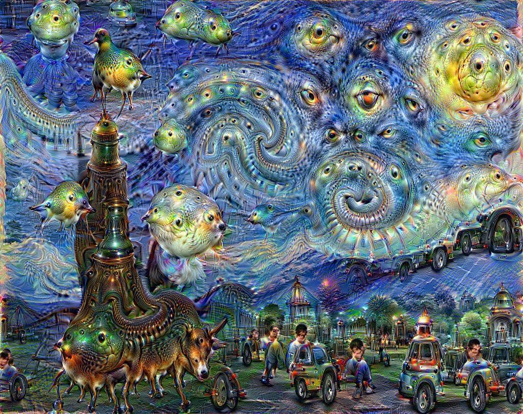 Figure 1: Deep Learning generated image.
In this first filmed session, we start by defining neural networks as a machine learning model inspired by the human brain, which arise as a way to create highly non-linear features in an intelligent way. We then show how predictions are computed via forward propagation. After that, we define the error function and the gradient descent algorithm to minimize it, which for neural networks makes use of an additional algorithm called backpropagation. Note that training a neural network requires a lot of training data in order to obtain a good approximation of the gradient at each point of the parameter space (and because there are a lot of parameters in a network, it is a high-dimensional space). The backpropagation algorithm leads to a much more efficient computation of the gradient compared to a direct method.
Neural Networks for supervised learning
The remainder of this post focuses on how to use a neural network for supervised learning problems. We start with a dataset with D input features composed of examples (rows) which we treat as column vectors x = (x1, x2, …, xD)T that we will use to teach our network. Note that the target column which indicates what the correct output should be for each example (needed by the network to learn) is not included in this vector. The motivation of neural networks is the need for an inherently non-linear model which is able, for instance, to perform well in classification problems where the decision boundary between the classes is non linear. Although linear models fed with non-linear transformation of the features (like powers or products between features) also exhibit non-linear boundaries, this rapidly becomes unfeasible when the number of features of the data grow.
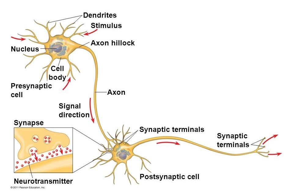
Figure 2: two interconnected human neurons
Neural networks are inspired by how the human brain works: it is composed of simple neurons, each carrying a simple computation with its inputs and transmitting its output to another neuron (Fig. 2). Similarly, neural networks consist of simple units called artificial neurons (Fig. 3(a)) which apply some non-linear function g (called activation function) to a linear combination of its inputs. The coefficients ? of the linear combination represent what the neuron has learned. The most commonly used activation function is the sigmoid.
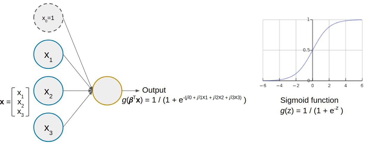 Figure 3: an artificial neuron with three inputs (left) and the sigmoid activation function (right)
A neural network is composed of multiple interconnected artificial neurons organized in layers, such that the outputs (a.k.a. “activations”) of the neurons of one layer act as inputs for the neurons of the next layer. Therefore, what the neurons in the inner layers are using as features (i.e. the activations from previous layer) are indeed non-linear combinations of the original input features. Such combinations possibly represent higher-level concepts (let’s call them mysterious features), instead of the raw features present in our data.
Multilayer perceptron and forward propagation to make predictions
If we number the neurons of the network, the output (predictions) of a fully connected network like the one displayed in Fig. 4 can be computed as shown in the image – this process is sometimes known as forward propagation. The notation and operations seem a bit ugly (a.k.a. “more technical”), but feel free to skip the figure if you are not interested in the maths. It is nothing more than applying the equation of Fig. 3 repeatedly for each neuron in the hidden layer and in the output layer. In the figure we are collecting together the parameters of each layer in matrices B(j). We call the set of all of these matrices B – that’s why the output of the network is a function of the inputs named hB.
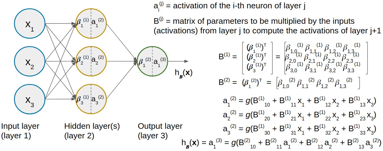
Figure 4: a fully connected network (multilayer perceptron) with one hidden layer and three inputs for examples with D = 3 features.
In case we are facing a binary classification problem, the class is determined by re-coding the output to one of the classes, either setting a threshold on the output (binary classification) or having as many neurons in the output layer as classes in our problem (multiclass classification). The output class computed by the network corresponds to the index of the neuron of the output layer which yields the highest output value.
Training algorithm: cost function and gradient descent via backpropagation
In any Machine Learning model, fitting a model means finding the best values of its parameters. The best model is one whose parameter values minimize the total error with respect to the actual outputs on our training data. Since the error depends on the parameters chosen, it is a function of the parameters, called the cost function J. The most common error measure is the MSE (Mean Squared Error):  where h?0, ?1, …, ?P is the equation of the model (be it a neural network or any other machine learning model) depending on P+1 parameters, and m is the number of training examples.
If the cost function is convex, it only has one global optimum, which is the global minimum. It can be found by computing the partial derivatives of J with respect to every variable (gradient vector ?J), and solving an equation system to find the point where the derivatives are all equal to 0 simultaneously (exact solution). Unfortunately, this can be difficult when the model equation is complicated (which yields a non-convex error function with many local optima), has many variables (large equation system) or is not derivable. That’s why we often use some approximate, iterative optimization algorithm for this task, which does not guarantee the global minimum but generally performs well. Gradient descent is the most common, although there is a wide family of techniques which share the approximate, iterative nature (getting closer and closer to the solution at each time step t) and the need for evaluating the partial derivatives of J at different parameter points ?(t).
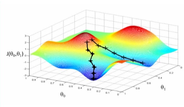
Fig 5: a plot of an error function J for two parameters and the iterative process of reaching a minimum (called “convergence”). Note the starting point heavily affects the solution obtained.
In our particular case, the parameters would be the set of matrices B composed of all the weights (betas) of the network. The equation of the output of a neural network is a highly complex and non-linear function of the inputs (more complex with more hidden layers), so it is really difficult to evaluate the partial derivatives. But there is a special way to compute and evaluate them at each point when training a neural network, called the backpropagation algorithm. Although it is a bit tricky to explain here, the intuition behind it is to partition the network’s error on a given train example among the neurons, to obtain how much each neuron has contributed to the total error on that example. This is done for every example from the output layer, back to the hidden layers until we reach the input layer, so it is like back-propagating the error from the output to the input neurons. Once backpropagation has been applied to evaluate the partial derivatives at the current point, the optimization algorithm uses them to update the network’s weights (betas) and moves on to the next iteration.
In the next session we will address the subject in a more practical way, taking a look at some of the parameters like activation functions and optimizers, and of course how to get our hands dirty and start creating our own deep neural nets, using TensorFlow and Keras.
Watch the video: Deep Learning Tutorial – Introduction to neural networks (Spanish)

