
Welcome back to our series on Swarm Intelligence Metaheuristics for Optimization! In part 1, we talked about a family of metaheuristic algorithms known generically as Ant Colony Optimization (ACO), which were specially well-suited for combinatorial optimization problems, i.e. finding the best combination of values of many categorical variables. Recall we define Metaheuristics as a class of optimization algorithms which turn out to be very useful when the function being optimized is non-differentiable or does not have an analytical expression at all.
We had framed ACO in the broader context of Swarm Intelligence, a yet-more-general family of algorithms able to solve hard optimization problems by a set of very simple cooperative agents and the appropriate communication rules between them, which together exhibit intelligent behaviour. In this post, we focus on another subclass of Swarm Intelligence algorithms, known as Particle Swarm Optimization (PSO), first published in 1995 at Univ. of Washington and Indianapolis [1].
Particle Swarm Optimization
Like ants, birds are another example of social animals which rely on each other to solve problems. But differently from ants, they are not blind so they can see each other and interact directly: a flying bird knows the position of its nearest birds. When searching for food, a bird does not know the exact location of the food but can perceive the distance to it. Ideally every bird would trust its neighbour birds if they are closer to the food.

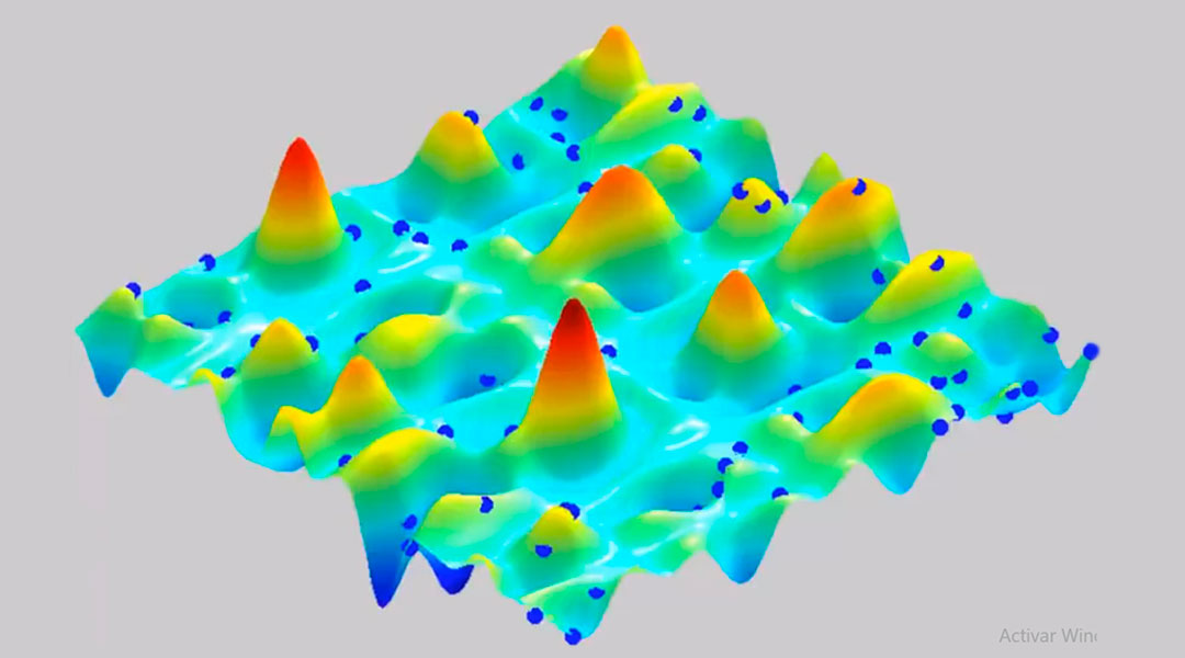
In a function optimization context, each bird is represented by a particle moving along the optimization space (which we assume either ℝn with n the number of variables being optimized, or a bounded subset of it). We initialize a number of particles (this number is problem-dependent and has to be tuned) spread along the space (Fig. 2), either randomly placed or following a uniform grid covering the feasible space in case it is bounded. Each particle is located at some point, which is a solution to the problem (not necessarily optimal) and it is in continuous movement during the algorithm, always exploring other solutions.
While ACO algorithms follow a constructive approach (each ant needs several steps to build a solution, which consists of a sequence of decisions of candidate values, one for each variable), each particle in PSO represents already a full solution in ℝn. In contrast with classical techniques like gradient descent, the particles do not use an analytical expression of the function to decide where to move next (as such expression might not even exist), but only the quality of the solutions of their neighbours. Such neighbour solutions are known to the particle. In addition, PSO is used mainly for continuous optimization problems, while ACO works best in combinatorial optimization (although continuous variants also exist).
Particles initialization and movement in PSO
We could somehow assume that a bird’s movement is guided by its current velocity (as it cannot turn suddenly), the position of its neighbours and how desirable each of the neighbour positions are, which is the analogy of the quality of the solutions found by such neighbours.
More formally, each particle i stores:
- A position xi ∈ ℝn which represents a solution
- A velocity vector vi ∈ ℝn representing its movement
- A real value fitnessi representing the value of the function at this point: fitnessi = f(xi). Recall f does not need to have a mathematical expression, it could be just a procedural function written in some programming language.
- Its best solution found so far, pBesti ∈ ℝn
- The fitness of its best solution, pBest_fitnessi = f(pBesti)
Therefore, for i = 1 … M (where M is the number of particles), the initial positions xi and the initial velocities vi of the particles are randomly initialized. Velocities should belong to an interval [-Vmax, Vmax]. The algorithm then updates the positions of the particles iteratively by applying the formulas:
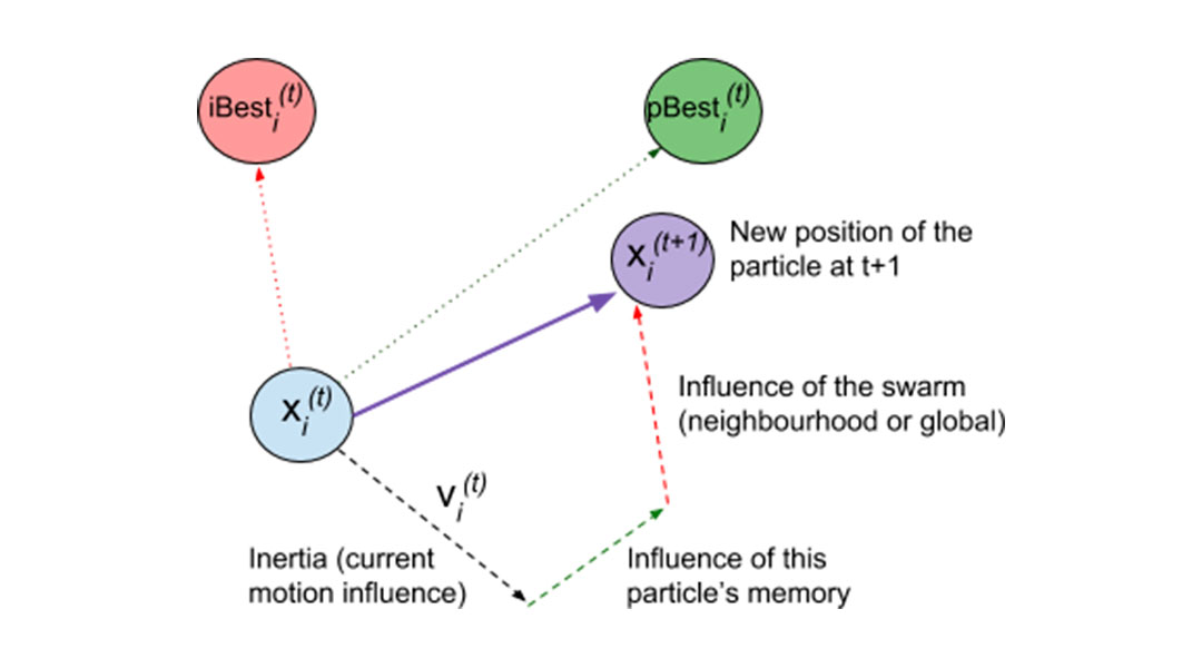
vi(t+1) = vi(t) + ?1 rand(n) .* (pBesti – xi(t) ) + ?2 rand(n) .* (iBesti – xi(t) )
xi (t+1) = xi(t) + vi(t+1)
Here, rand(n) ∈ [0,1]n is a random vector of n dimensions drawn from n uniform distributions U[0,1], and .* represents element-wise vector multiplication. Coefficients ?1 and ?2 are constant and stand for the weights given to the cognitive and the social component, respectively, whereas iBesti represents the best solution found by the neighbourhood of i. Another variant of the algorithm uses gBest instead, which stands for the global best solution found so far by the whole population. In that case, iBest would be replaced by gBest in the first equation. The diagram below represents the above equations as a graphical sum of vectors.
Finally, the particle must update iBesti after each iteration (or alternatively, every particle must update the global variable gBest whenever they find a better pBesti, in case we are using the global variant). The algorithm repeats this process until a maximum number of calls to the fitness function f() is reached.
PSO pseudocode (local neighbourhood variant)
INPUT:
M: number of particles of the swarm
OUTPUT:
best solution found by any particle of the swarm
- Initialization step:
For t := 0 to M
Initialize xi and vi randomly - While(there are fitness evaluations remaining)
a) t := t+1
b) For i :=1 to M
fitnessi = f (xi) # evaluate xi
IF fitnessi IS BETTER THAN pBest_fitnessi THEN
pBesti := xi
pBest_fitnessi := fitnessi - For i := 1 to M
vi (t+1) := vi(t) + ?1 rand(n) .* (pBesti – xi(t) ) + ?2 rand(n) .* (gBest – xi(t) )
xi (t+1) := xi(t) + vi(t+1) - RETURN gBest
PSO parameter tuning
- Swarm size M: between 20 and 40 particles. 10 particles for simple problems, and between 100 and 200 for very complex ones.
- Maximum velocity: Vmax is set according to the range of each variable
- Update ratios: generally ?1 = ?2 = 2
- Local vs Global PSO: the global version converges faster but tends to get trapped in local optima more easily.
A note on the neighbourhoods for the local variant
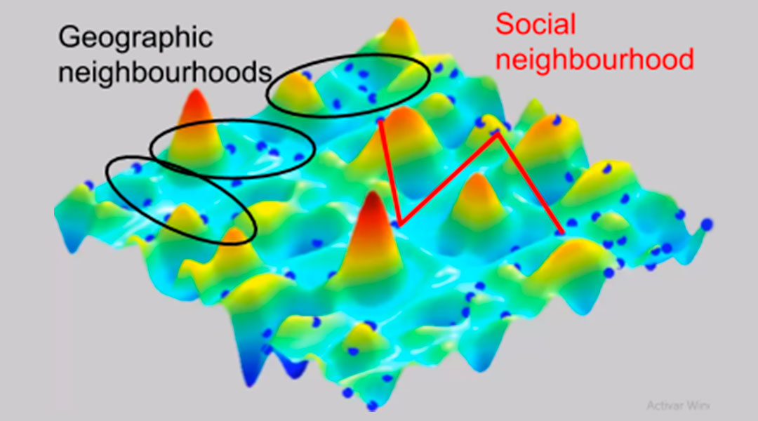
We have to define which particles are part of the neighbourhood. In the above pseudocode, this is represented by the call to best_particle_in_neighbourhood(i). There are two options (Fig. 4):
- Geographic neighbourhood: compute the distance to all the other particles and take the closest ones. This means the neighbourhood changes between iterations as the particles move during the algorithm.
- Social neighbourhood: a list of neighbours is defined for each particle at the beginning of the algorithm, and the lists do not change during the algorithm, no matter the relative positions of the particles. It is the most common neighbourhood. Very often, a ring structure is formed as a social neighbourhood. Particles are numbered just after initialization according to their positions, and a particle is assigned the particles that are consecutively before or after it in the numbered list.
Neighbourhood size: usually 3 or 5 particles is enough. It is not a very important parameter.
Other PSO variants proposed
It is very common that velocities grow too large and lead to a very fast movement along the space, missing good areas. It is important to set Vmax properly. Two variants have been proposed to remedy this problem:
- Setting an explicit inertial factor
- Setting a coefficient K that reduces the velocity after each update:
K = 2 / | 2 – ? – sqrt(?2 – 4?) | where ? = ?1 + ?2
Another parameter for which variants have been proposed is the swarm size. It can be dynamically adapted as follows:
- If the quality of the neighbourhood has improved but the particle is the worst of its neighbourhood, the particle is destroyed (it dies).
- If the particle is the best of its neighbourhood and there has been no improvement on the neighbourhood, a new particle is created from that particle.
- The decisions are made in a probabilistic way as a function of the current swarm size.
The neighbourhood size could also be adapted as a function of the swarm size. Finally, the weights ?1 and ?2 may also vary dynamically along the execution of the algorithm: the better the particle’s personal best, the larger the weight of the cognitive component, and analogously, the better the neighbourhood best solution, the larger the weight to go towards it.
Applications of PSO
PSO has been applied to a lot of optimization problems in engineering [2]. Many of them deal with finding the optimal distribution (positions) or setting for a device, for instance:
- Optimal placement of electronic components in VLSI (integrated) circuits to minimize the manufacturing cost
- Job scheduling problems [3]
- Power plant and power systems optimization
- Power and water demand estimation [4]
- Radar and antenna optimization [5]
References
[1] Kennedy, J. and Eberhart, R. Particle Swarm Optimization. Proc. of the IEEE International Conference on Neural Networks, 4:1942-1948 (1995).
[2] Erdogmus, P. (Editor). Particle Swarm Optimization with Applications. IntechOpen (2018).
[3] Ma, R. J., Yu, N. Y., and Hu, J.Y. Application of Particle Swarm Optimization Algorithm in the Heating System Planning Problem. The Scientific World Journal, vol. 2013, Article ID 718345 (2013).
[4] SaberChenari, K., Abghari, H., and Tabari, H. Application of PSO algorithm in short-term optimization of reservoir operation. Environmental Monitoring and Assessment 188 (12):667 (2016). 10.1007/s10661-016-5689-1.
[5] Golbon-Haghighi, M.-H., Saeidi-Manesh, H., Zhang, G., and Zhang, Y. Pattern Synthesis for the Cylindrical Polarimetric Phased Array Radar (CPPAR). Progress In Electromagnetics Research M, 66:87-98 (2018).


